Have you ever wanted to know how Monet would paint the landscape in front of you? Sadly, he’s not around to paint it anymore but Machine Learning can give us an idea of what he might have produced. To see the finished product and try converting your own images, head here.

Image-to-image translation has seen remarkable progress in recent years. Image translation involves producing a mapping network to convert an image from one style to another. However, most efforts have focused on datasets where paired images are available. CycleGAN (Zhu et al. 2020) represents a big shift forward in terms of unpaired image-to-image translation.

CycleGAN

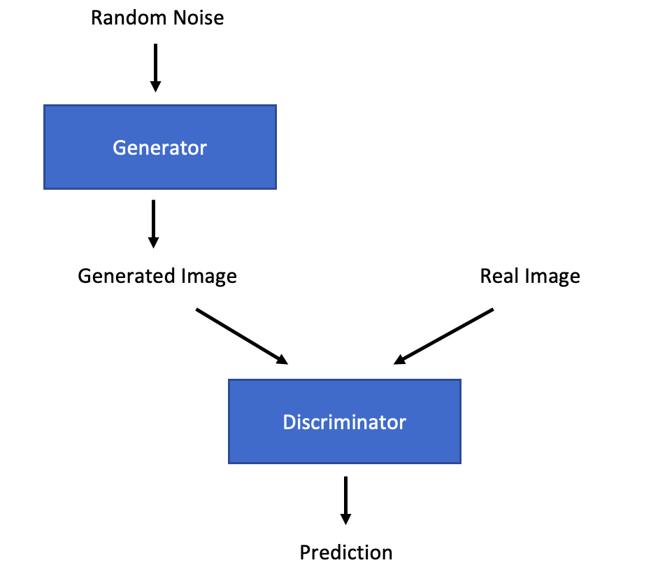
CycleGAN is based on a General Adversarial Network (GAN) framework (Goodfellow et al. 2014), where two models (a generator and discriminator) compete against one another. The generator attempts to produce a fake image that could have come from the target distribution. The discriminator then attempts to tell the difference between the real and fake images.

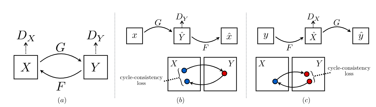
Training an image-to-image translation network using unpaired images represents a particularly difficult challenge because a generator may learn to predict an output image that can fool the discriminator into thinking it is part of the target distribution but the image may bear no resemblance to the original input. In order to ensure that the mapping network produces a viable image, a cycle consistency loss is included in the objective function. This ensures that, if a generated image is passed through the reverse generator function, the resulting image will be similar to the original image. This helps to ensure that the mapping function learns to produce the correct image.

(Zhu et al. 2020)

CycleGAN represents a framework for training image-to-image translation models. It does not require a specific framework for the generator or the discriminator. However, the original paper proposes the networks below.

The generator is based on this paper by Johnson et al. (2016). The first and final two layers downsample and upsample the image respectively so that the main model works with a smaller image to improve computational efficiency. All layers are based on convolutions and there are no fully connected layers. The central layers consist of residual blocks which add the input of that block to the output. This idea was originally put forward in this paper (He et al. 2015) and ensures that a deeper network will always outperform a shallower network as the resulting function classes at each layer are nested. Reflection padding rather than zero padding is used to remove edge defects and Instance norm is used instead of Batch norm.

The discriminator is based on a patch discriminator, first described as PatchGAN in this paper by Isola et al. 2018. The patch discriminator is a convolution based network which scans each ‘patch’ of the image and produces an output. The mean of all the outputs is taken and returned. The intuition behind treating the image in patches is firstly that it reduces the size and therefore the computation power needed for the model. However, this does not come at the expense of accuracy because the ability to discern between a fake and real image is largely concerned with small scale differences rather than the image as a whole. The authors found that 70x70 pixel patches were the most effective.

In a CycleGAN, two generators and discriminators are trained: one for the forward direction to map images from distribution A to distribution B, and another for the reverse direction to map from B to A. Both discriminators are trained as usual: to maximise the output when given a real image and minimise the output when given a fake image. The objective function for the generator contains two principle parts: first is the standard generator loss function (to maximise the output from the discriminator of a generated image) and second is the cycle consistency loss function (as explained above). The latter function minimises the L1 norm of the resultant vector between the original image and the reconstructed image that has been passed through both generators.

(Zhu et al. 2020)

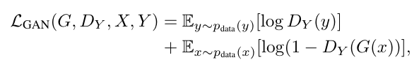
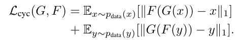
For the generator update step, the GAN loss (first equation) is minimised, where x is the input image, G is the generator and D is the discriminator. In practice the loss function does not use the negative log likelihood but instead the square difference. In addition, the generator update step contains the cycle consistency step (second equation) which passes both inputs (x and y) through both generators (G and F) in turn and then minimises the difference between the two (L1 norm). This step is then multiplied by a scalar value (10 in the original paper) to increase its weighting in the overall loss function (third equation). The discriminator loss involves maximising the GAN loss (first equation). The cycle consistency loss is not included in the discriminator loss.

GANs are notoriously temperamental to train. One method to stabilise training is using a Wasserstein GAN. However, the authors of the CycleGAN paper propose other methods to stabilise training. Firstly, for the discriminator and the first part of the generator loss, the squared difference is calculated rather than using the negative log likelihood. Second, the L1 norm is used rather than the L2 norm for the cycle consistency loss. Third, in order to prevent model oscillations, a buffer of images from the previous set of generators is used rather than taking images from the current generator. Finally, for photo-to-painting tasks, the authors recommend including an identity loss in the generator objective function. Here, the generator is passed a target image as the input and the L1 norm of the resultant between the generated image and the original image is minimised.

(Zhu et al. 2020)

The identity loss takes an image from the target dataset and feeds it through the generator. The difference between the original (y) and the resulting image (G(y)) is then minimised (L1 loss). The same is repeated for the other direction (x and G(x)) and the two losses added.

Implementation

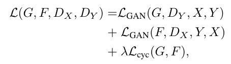
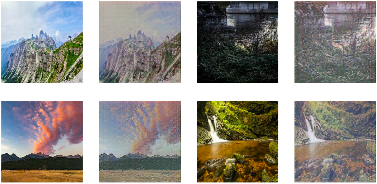
You will find my code implementation of CycleGAN for tackling the Kaggle “I’m something of a Painter Myself” challenge here. The aim is to convert landscape photos into Monet-style paintings. Here is a sample of some of the generated images (right) alongside their input photos (left):

To try it out with your own images, head here.

This implementation follows the model used in the original CycleGAN paper as closely as possible. The use of an image buffer greatly improved training stability. During every batch a random generated image is added to the buffer and the oldest image removed. A random sample from the image buffer is fed to the discriminator on each occasion.

Kaggle provides a dataset of landscape photos and Monet paintings. The landscape photos were downloaded from the internet and some of the images made training more difficult: there were several black and white images which the model struggled to add colour to. Some of the images were circular and the model struggled to fill in the resulting whitespace. In general, the model produced plausible images. The major issue was image resolution as the produced images are noticeably blurry. Monet’s style helps to mask this slightly as his brushstrokes also give off a slightly blurry feel. The difference is therefore most noticeable in the photo generator. As described in Isola et al, 2018, the likely reason for this is the use of L1 loss in the objective function which is known to result in blurring. However, the Discriminator loss should, theoretically, act to mitigate this effect. It is plausible that, with further training, the blurring would be reduced, especially given the high quality of the images produced in the original paper and the fact that this implementation follows the original very closely.

Initially the model stopped training as the generator loss kept climbing due to the increased capability of the discriminator. Interestingly this affected the forward direction more than the reverse direction, perhaps as a result of the larger variety of images found in the photo set compared to the Monet set and the fact the Monet dataset contains fewer, more similar images and it is hence easier for the discriminator to identify them. To combat this, a decaying mean value (lambda = 0.8) for the generator loss was kept and the discriminator training step was only carried out if the generator loss was below a key value (0.5). Training then proceeded smoothly. The model was run for approximately 2.5 hours (125 epochs) on one GPU.