What is Machine Learning and what is a Neural Network?
Traditional programming involves writing code that then gets executed. Everything that the program does has to be clearly written out in code. This can be used to make predictions. For example: say you want to predict what the price of a house should be. You could specify some inputs (e.g. number of bedrooms, location, etc.) and then predict a price. However, there would need to be some logic in the middle and you would need to come up with it. For example, you might come up with a simple formula that combines the number of bedrooms with the distance from the city centre. When you run the program it simply uses your logic. This is still useful: computer programs run incredibly quickly and so, if you need to make lots of predictions, it’s a great help, but it relies on your understanding of how inputs are related to an output. What if it could draw its own connections?
Machine Learning aims to build a program that can teach itself the relationships between things. The program consists of a model that makes predictions. The model is then given some inputs and makes a prediction. It then compares that prediction to the real output and, if it is wrong, updates itself to make it more likely to predict correctly in the future. This way you do not need to explicitly tell the model how to interpret the data and how to draw connections, it does it itself.
Neural networks are just one machine learning method. Other methods, e.g. decision trees, not only exist but are indeed better for certain applications. However, neural networks have attracted significant attention because they seem to be the best solution to a large portion of the problems that machine learning can solve.
Neural Networks
In the following simple example we will follow all of the steps necessary to train a network:
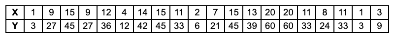
The relationship we are going to learn is a very simple linear relationship. However, initially we do not know the relationship, we just have some data:
Define the model
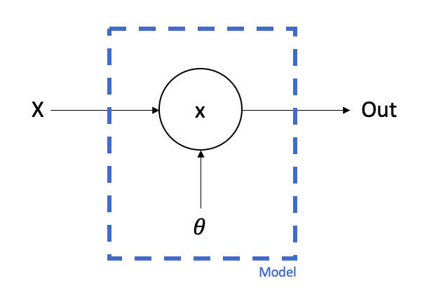
A neural network is essentially a set of numbers (called parameters) and a sequence of operations for how those numbers should interact with the input in order to produce the output. These operations are generally very simple but, when combined at scale, can have very powerful predictive properties.
The neural network we will use is the simplest possible: it consists of just one parameter. The sequence of operations is just going to be to multiply the input by our parameter value to give the output.
To start with we need to initialise the value of our parameter. We could choose pretty much anything but let’s choose 1.
Make a prediction
This step is usually called the ‘forward pass’.
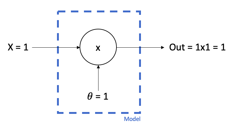
We then pass our first bit of data to the model, in this case x=1 and y=3.
Our model takes the x value, multiplies it by the parameter value and produces a predicted value. In this case: 1x1 = 1
Measure the accuracy
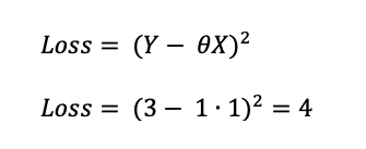
We then need an objective function (sometimes called a loss function) to tell how closely our prediction matches the target. In this case our loss function would simply calculate the squared difference between the prediction and the target value. This result is called the ‘loss’. We want our loss to be as small as possible because, when the loss is zero, it means our prediction is the same as our target.
Assess how each parameter affects the prediction
This step is usually called the ‘backward pass’.
Here, we identify how the loss is affected by the parameter value. If we increase the parameter value slightly, does it increase the loss or decrease it? We therefore need to differentiate the Loss with respect to the parameter. Our overall function and its derivative is as follows:
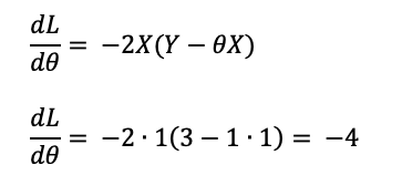
In this case we just have one parameter so we only need to do this once. However, for a larger model you would need to calculate all of the partial derivatives and update every single one.
In this case the derivative of the loss with respect to the parameter is -4. Let’s take a step back and understand what that means. If we increase the value of the parameter very slightly then we would expect that to cause the loss to decrease. If we decrease the value of the parameter then the loss would increase.
Update the parameters
This process is usually called ‘gradient descent’.
We now need to update the parameter so that it will make a better prediction next time. The gradient tells us which direction we should move the parameter in, but how much should we change it? This is determined by a constant called the ‘learning rate’ which is decided by the user. The size of this constant greatly affects the learning process and is something to tweak in order to improve the efficiency with which the model learns.
We will use a learning rate of 0.001 in this example.
Because we want the loss to decrease we therefore want to subtract the gradient from the parameter value. We will therefore use the following equation to update the parameter:
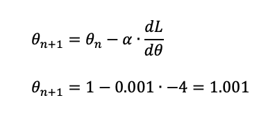
In this case 1 - 0.001x(-4) = 1.004. Our new value for our parameter is 1.004. Notice that if we had chosen a larger learning rate then it would have made a larger jump. However, then we run the risk of overshooting.
Repeat
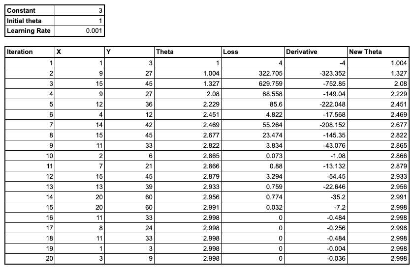
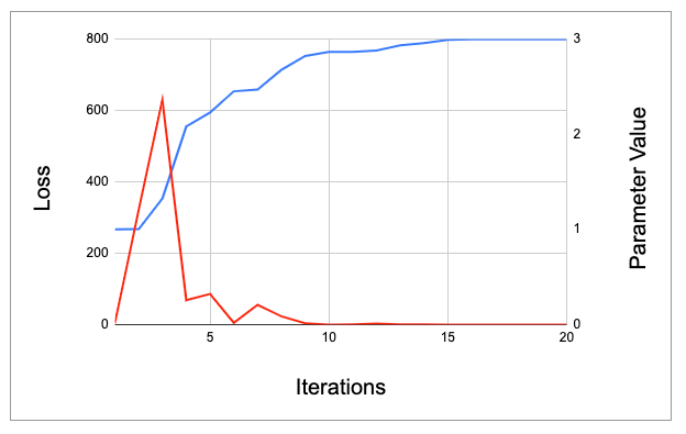
Our parameter has indeed got closer to the value we are hoping for (3) but it’s still not particularly close. We’ll need to repeat this process multiple times before we are able to make accurate predictions. See the table and graph below:
Linear Network
This is in essence what a neural network is doing. However, for our model to have more powerful predictive capacity we need more parameters. This is where some knowledge of linear algebra and matrix multiplication is useful. A linear network (still a relatively simple kind of network) consists of a number of layers. Each layer consists of two sets of parameters (weights and biases) and does the following:
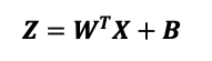
Where X is an Nx1 dimensional input vector, W is an NxM dimensional matrix and B is an Mx1 dimensional vector
The incoming values are multiplied (matrix multiplication) by a set of weights and then added to a set of biases. This produces a new set of values which can be passed to the next layer.
Activation function
Two successive matrix multiplications can always be represented by one multiplication. This is because matrix multiplications are linear transformations. As a result, adding more layers to our model doesn’t guarantee that our model becomes more capable. We therefore need to introduce a ‘non-linearity’ or activation layer that breaks the linear relationship and allows the model to learn more complex functions. This function can be very simple, for example the ReLU function which keeps all positive values the same but replaces all negative values with zero. This is enough to break the linearity and improve the model’s performance.
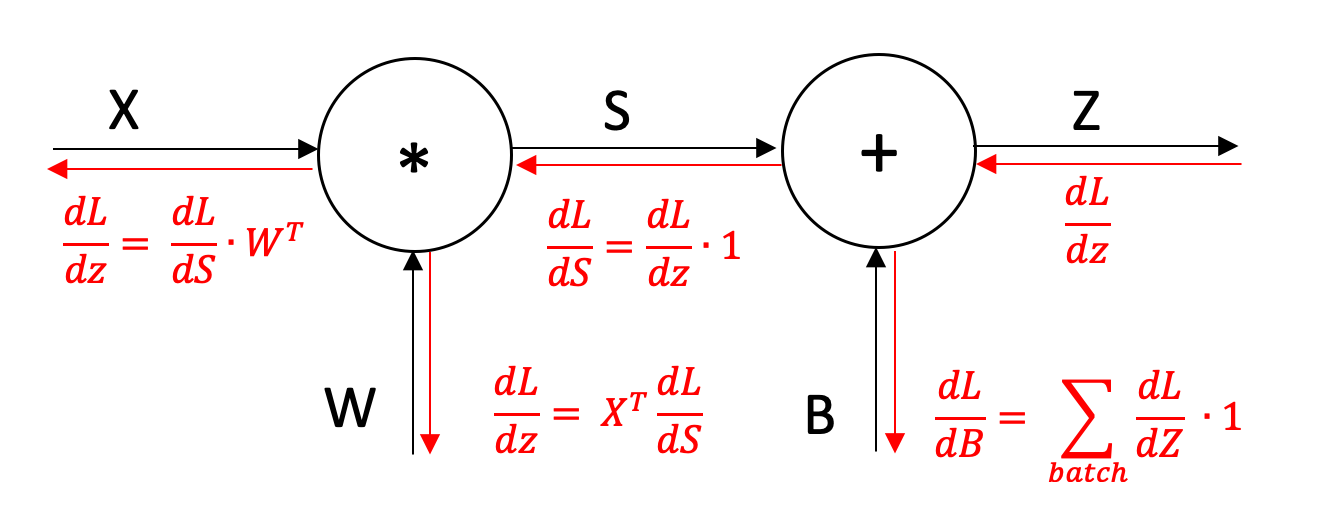
Backpropagation in linear networks
When we have multiple layers in our network working out how one parameter affects the loss is more difficult because most parameters do not affect the loss directly. However, we can use the chain rule to work backwards and multiply each of the derivatives together.
Summary
This was a very high level introduction to Neural Networks and Machine Learning. Hopefully it has given you some idea about the essence of what a neural network is doing. There is lots more to learn and I’ve tried to include key terms so that you can go away and read more about them. If you're interested in learning more about Machine Learning and aren't sure where to get started head over to this other post.