Using and implementing a Neural Network could not be easier these days. Not only are there optimised GPU capable ML libraries like PyTorch and Tensorflow that can run your code many times faster, these libraries also make the job of writing the code so much easier with custom functions that take care of many aspects under the hood. The largest of those is probably gradient tracking and backpropagation which essentially takes place without you even thinking about it. This is without mentioning additional libraries built on top of this (e.g. FastAI) which make it even easier, or sites like Hugging Face which allow you to essentially plug and play models. This begs the question: why would anyone want to start from scratch and code up a neural net in Numpy? Well, in reality, no-one does. However, it’s an excellent exercise in improving your understanding about what goes on under the hood and I would certainly highly recommend it to anyone starting out. It also allows you to dive deep into the network and explore what’s going on, a great way to understand what your model is doing and help it to seem like less of a black box.
What are we building?
This article walks you through how to build a simple multilayer perceptron with a customisable size. We’ll include two activation functions (Sigmoid and Leaky ReLU) and we’ll add the option for Batch Normalisation. We’ll also include two loss functions: Mean Square Error and Cross Entropy, to use depending on what task we want to assign our model to. We’ll then examine how it does on MNIST and compare it to an identical model built in PyTorch.
The code for this project is available on GitHub in a Jupyter notebook.
This article assumes that you are already familiar with Machine Learning and understand the general process (for a high level introduction see here). The focus is mainly on implementation and so some mathematical aspects, e.g. derivatives, are not explained fully. However, I have tried to include links for further reading.
Step 1: Creating the Class
First, install dependencies:
              import numpy as np
              import pandas as pd
              import matplotlib.pyplot as plt
              from PIL import Image
Our model class will need to take a number of parameters, most importantly the dimensions of the network and the learning rate. In this case the dimensions should be passed as a list of integers determining the input size for each layer (and the final output size). We’ll also pass some additional settings so that we can select the loss and activation functions we want to use, as well as if we want to use batch normalisation. We then store these variables and select the correct loss function and activation function (along with its derivative function). We will define all of these functions later. Finally, we’ll also call a function to create the model, which initialises all of the weights and creates variables to store the gradients and activations as they get passed through the network.
              class Model():
                def __init__(self, model_dimensions, lr=0.01, activation="Leaky ReLU", loss="Cross Entropy", use_batch_norm=True)
                  self.dims = model_dimensions
                  self.lr = lr
                  self.layers = len(model_dimensions) - 1
                  self.use_batch_norm = use_batch_norm
                  self.train_mode_on = True
                  if loss == "Cross Entropy":
                    self.loss = self.cross_entropy
                  elif loss == "MSE":
                    self.loss = self.MSE_loss
                  else:
                    raise Exception("Loss must be either 'Cross Entropy' or 'MSE'")
                  if activation == "Sigmoid":
                    self.activation = self.sigmoid
                    self.activation_backwards = self.sigmoid_backwards
                  elif activation == "Leaky ReLU":
                    self.activation = self.Leaky_ReLU
                    self.activation_backwards = self.Leaky_ReLU_backwards
                  else:
                    raise Exception("Activation function must be either 'Sigmoid' or 'Leaky ReLU'")
                  self.parameters, self.activations, self.gradients, self.bn = self.create_model()
We only want to store gradients when we are training the model and batch normalisation works differently during training and test modes. We therefore need to create a variable (train_mode_on) to define the state of the model. The first two functions we’ll create, train_mode() and test_mode(), are therefore simply to allow us to easily toggle between modes.
              def train_mode(self):
                  self.train_mode_on = True
                def test_mode(self):
                  self.train_mode_on = False
Step 2: Create the Model
Here, we create several dictionaries to store and keep track of the weights, activations and gradients for our network. We iterate through each layer and create a corresponding weight and bias matrix, along with an identical matrix to store the gradients. We also need to initialise the weights. We’ll follow how PyTorch does this.

pytorch.org
              def initialise_weights(self, size):
                  param = 2*np.random.random(size) - 1
                  stdv = 1. / np.sqrt(size[0])
                  return param * stdv
We also do the same for the gamma and beta factors in the batch normalisation layer. These are initialised to 1 and 0 respectively so that initially they have no effect on the normalisation. The running mean values for the mean and variance are initialised to 1 and 0 too (more on batch normalisation later).
              def create_model(self):
                  parameters, activations, gradients, bn = {}, {}, {}, {}, {}
                  gradients['L'] = None
                  for layer in range(1,len(self.dims)):
                    input = self.dims[layer-1]
                    output = self.dims[layer]
                    parameters['W'+ str(layer)] = self.initialise_weights((input,output))
                    parameters['B'+ str(layer)] = self.initialise_weights((output,))
                    parameters['gamma' + str(layer)] = np.ones(output)
                    parameters['beta' + str(layer)] = np.zeros(output)
                    bn['mu' + str(layer)] = np.zeros(output)
                    bn['var' + str(layer)] = np.ones(output)
                    gradients['W'+ str(layer)] = np.zeros((input,output))
                    gradients['B'+ str(layer)] = np.zeros(output)
                    gradients['gamma' + str(layer)] = np.zeros(output)
                    gradients['beta' + str(layer)] = np.zeros(output)

                  return parameters, activations, gradients, bn
Finally, following the same protocol as PyTorch, we’ll set the default behaviour to involve adding gradients to stored gradients when we do the backward pass rather than always replacing them. As a result, we’ll need a function to zero the gradients.
              def zero_grad(self):
                  self.gradients['L'] = None
                  for layer in range(1,self.layers+1):
                    self.gradients['W'+ str(layer)] = self.gradients['W'+ str(layer)] * 0
                    self.gradients['B'+ str(layer)] = self.gradients['B'+ str(layer)] * 0
                    self.gradients['gamma' + str(layer)] = self.gradients['gamma' + str(layer)] * 0
                    self.gradients['beta' + str(layer)] = self.gradients['beta' + str(layer)] * 0
Step 3: Activation layers
We’ll include the option to use two activation functions: Sigmoid and Leaky ReLU (the latter can also function as a simple ReLU by setting the alpha value to 0). The sigmoid function takes the input and squeezes it between 0 and 1. It is defined as follows:

                def sigmoid(self, x):
                    return 1/(1+np.exp(-x))
We will also need the derivative function for the backward step:
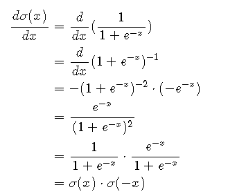
                def sigmoid_backwards(self, dx, x):
                    sig = self.sigmoid(x)
                    return dx*sig*(1-sig)
The ReLU function (Rectified Linear Unit) leaves values greater than zero unchanged but returns zero for all values less than zero. Leaky ReLU does the same but instead multiplies negative values by an alpha value (usually very small, e.g. 0.01). This helps the model to train by ensuring that all values have a gradient and can therefore be updated during the backpropagation step (avoiding the “dying ReLU” problem). Leaky ReLU is defined as follows:
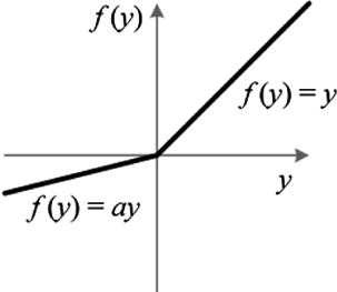
                def Leaky_ReLU(self, x, alpha=0.01):
                    return np.maximum(alpha*x,x)
The derivative is simply 1 when x > 0 and alpha when x < 0. Technically it is undefined at 0 but we will simply define it to be 1 in order to avoid numerical issues.
                def Leaky_ReLU_backwards(self, dx, x, alpha=0.01):
                    return dx*np.where(x<0,alpha,1)
Step 4: Batch normalisation
Batch normalisation greatly increases training stability of deep neural networks. If we imagine a network which is designed to classify images, we can see that the top left hand pixel of the image is always going to follow the same path through the network regardless of which image we use. Therefore, when we pass a batch of images through the network during training, all of the values in the same position along the batch dimension pass through the network in the same way. Normalising these values greatly improves training.
In short: it normalises along the batch dimension and then re-scales the distribution with two learnable factors: gamma and beta. The equation is given below.
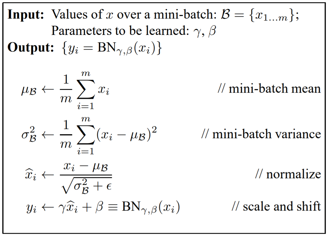
(Ioffe and Szegedy, 2015)
The intermediate steps need to be cached for the backward pass. We also need to differentiate between training and test modes. This is because, during testing we want to normalise according to the distribution the model learned with during training. As a result, we need to keep a running mean of the mean and variance during training and store this for use during testing (‘mu’ and ‘var’ in the code).
                def batch_norm_forward(self, x, layer, eps=1e-5):
                    N, D = x.shape
                    gamma = self.parameters['gamma' + str(layer)]
                    beta = self.parameters['beta' + str(layer)]
                    if self.train_mode_on:
                      mu = 1./N * np.sum(x, axis = 0)
                      xmu = x - mu
                      var = 1./N * np.sum(xmu ** 2, axis = 0)
                      self.bn['mu' + str(layer)] = 0.9 * self.bn['mu' + str(layer)] + 0.1 * mu
                      self.bn['var' + str(layer)] = 0.9 * self.bn['var' + str(layer)] + 0.1 * var
                    else:
                      mu = self.bn['mu' + str(layer)]
                      xmu = x - mu
                      var = self.bn['var' + str(layer)]
                    sqrtvar = np.sqrt(var + eps)
                    ivar = 1./sqrtvar
                    xhat = xmu/sqrtvar
                    gammax = gamma * xhat
                    out = gammax + beta
                    if self.train_mode_on:
                      self.bn['cache' + str(layer)] = (xhat,xmu,ivar,sqrtvar,var,eps)
                    return out
The backward pass involves numerous steps and can be best understood by drawing a computational graph to represent the whole process. An excellent overview can be found here.
                def batch_norm_backward(self, dx, layer):
                    (xhat,xmu,ivar,sqrtvar,var,eps) = self.bn['cache' + str(layer)]
                    gamma = self.parameters['gamma' + str(layer)]
                    N,D = dx.shape
                    self.gradients['gamma' + str(layer)] += np.sum(dx*xhat, axis=0)
                    self.gradients['beta' + str(layer)] += np.sum(dx, axis=0)
                    dxhat = dx * gamma
                    divar = np.sum(dxhat*xmu, axis=0)
                    dxmu1 = dxhat * ivar
                    dsqrtvar = -1. /(sqrtvar**2) * divar
                    dvar = 0.5 * 1. /np.sqrt(var+eps) * dsqrtvar
                    dsq = 1. /N * np.ones((N,D)) * dvar
                    dxmu2 = 2 * xmu * dsq
                    dx1 = (dxmu1 + dxmu2)
                    dmu = -1 * np.sum(dxmu1+dxmu2, axis=0)
                    dx2 = 1. /N * np.ones((N,D)) * dmu
                    dx = dx1 + dx2
                    return dx
Step 5: Forward pass
Now we are ready to use our model and create the forward pass. Now that we have everything in place this is relatively straightforward. For every layer, we multiply the previous activations by the weights and add the biases. We then apply batch normalisation (if activated) and finally pass through the activation layer to give the new activations. We need to make sure we store these activations for the backward pass.
                def forward(self, x):
                    self.activations['A0'] = x
                    for layer in range(1,self.layers+1):
                      Z = self.activations['A'+ str(layer-1)] @ self.parameters['W'+ str(layer)] + self.parameters['B'+ str(layer)]
                      self.activations['Z'+ str(layer)] = Z
                      if self.use_batch_norm:
                        Z = self.batch_norm_forward(Z, layer)
                      self.activations['A'+ str(layer)] = self.activation(Z)
                    return self.activations['A'+ str(self.layers)]
Step 6: Loss function
Once the model has made a prediction we need a metric to measure its success. We’ll implement two possible loss functions depending on what kind of problem we are applying our model to. For a regression problem we will want to use mean square error (MSE) and for a classification problem we’ll want to use cross entropy with softmax. We will calculate the gradient of the loss ahead of time and store it ready for the backward pass. For more information on loss functions see this previous post.
Mean Square Error
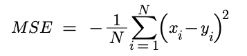
                def MSE_loss(self, x, y):
                    self.gradients['L'] = 2 * (x - y) / y.shape[0]
                    return np.mean((x-y) ** 2)
Cross Entropy with Softmax
Softmax is applied first to convert each activation into a probability. The cross entropy is then calculated to assess how similar the predicted distribution is to the target distribution. The derivative involves a number of steps but simplifies incredibly nicely. For a detailed overview, head here.
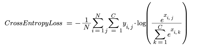
                def cross_entropy(self, x, y):
                    exps = np.exp(x)
                    s = exps / np.sum(exps,axis=1,keepdims=True)
                    loss = np.mean(np.sum( y * -np.log(s), axis=1))
                    self.gradients['L'] = (s - y) / y.shape[0]
                    return loss
Step 7: Backward pass
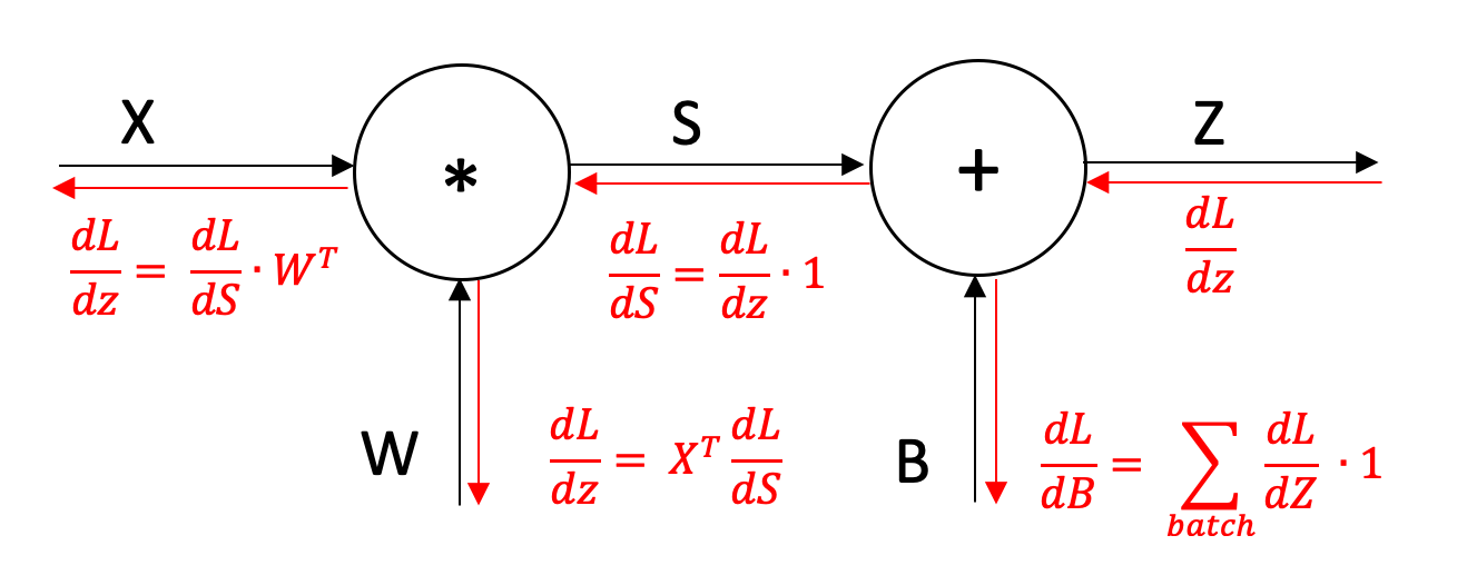
We now need to backpropagate through the network and calculate the gradients for each parameter. At each stage we apply the chain rule and multiply the local gradient by the gradient of the loss with respect to the current position to move one more step backwards in the network. We start by taking the gradient of the loss that we have already calculated. We have already built functions to calculate the derivative of the activation layers and the batch normalisation layers so these steps are relatively straightforward.
For the linear layer, we need to calculate the derivatives for the weights and biases, as well as for the input so that it can be passed to the next layer. The derivatives are stored so that we can use them to update the parameters later on. The derivatives are given as follows:
                def backward(self):
                    dZ = self.gradients['L']
                    for i in range(self.layers):
                      layer = self.layers - i
                      dA = self.activation_backwards(dZ,self.activations['Z'+ str(layer)])
                      if self.use_batch_norm:
                        dA = self.batch_norm_backward(dA, layer)
                      self.gradients['B'+ str(layer)] += np.sum(dA,axis=0)
                      self.gradients['W'+ str(layer)] += self.activations['A'+ str(layer-1)].T @ dA
                      dZ = dA @ self.parameters['W'+ str(layer)].T
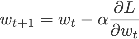
Step 8: Update the parameters
Once the gradients have been calculated, the next step is to perform gradient descent and update the parameters. We will use simple stochastic gradient descent (SGD) rather than any more advanced optimiser. This simply multiplies the gradient by a constant (the learning rate) and then updates the parameter by subtracting this value. Remember that each gradient is the gradient of the loss with respect to that parameter. Therefore by subtracting the gradient the parameter is updated in a way that should reduce the loss, hence improving the accuracy of the model.
                def step(self):
                    for layer in range(1,self.layers+1):
                      self.parameters['W'+ str(layer)] -= self.lr * self.gradients['W'+ str(layer)]
                      self.parameters['B'+ str(layer)] -= self.lr * self.gradients['B'+ str(layer)]
                      self.parameters['gamma'+ str(layer)] -= self.lr * self.gradients['gamma'+ str(layer)]
                      self.parameters['beta'+ str(layer)] -= self.lr * self.gradients['beta'+ str(layer)]
Step 9: Training loop
By now the model is essentially built but we can add some additional helper functions to make training a bit easier. During training, we need to loop through the data loader (see below) to get each batch of training examples. The first step is to zero the gradients so that we are not adding the new gradients to the previous ones. Then we perform our forward pass, calculate the loss and perform our backward pass, then update the parameters and store the losses to plot later.
                def train_model(self, dataloader):
                    losses = []
                    self.train_mode()
                    iterator = iter(dataloader)
                    for batch in range(len(dataloader)):
                      x,y = next(iterator)
                      self.zero_grad()
                      out = self.forward(x)
                      loss = self.loss(out,y)
                      self.backward()
                      self.step()
                      losses.append(loss)
                    return losses
To test the accuracy of our model we need to use the test examples that we have set aside. Here, we complete the forward pass on each batch and then assess whether the prediction made by the model is correct. This can then be compiled to give an overall accuracy score.
                def test_model(self, dataloader):
                    count = 0
                    self.test_mode()
                    iterator = iter(dataloader)
                    for batch in range(len(dataloader)):
                      x,y = next(iterator)
                      out = self.forward(x)
                      count += np.where(np.argmax(out,axis=1) == np.argmax(y,axis=1), 1, 0).sum()
                    accuracy = 100* count / (len(dataloader)*x.shape[0])
                    return accuracy
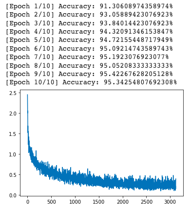
Combining this altogether we can create an overall training program which first completes a training loop, then calculates the accuracy and repeats for a given number of epochs. We can then plot the losses at the end.
                def train(self, train_dataloader, test_dataloader, epochs=1):
                    losses = []
                    for epoch in range(epochs):
                      epoch_losses = self.train_model(train_dataloader)
                      losses = np.concatenate((losses, epoch_losses))
                      accuracy = self.test_model(test_dataloader)
                      print(f'[Epoch {epoch+1}/{epochs}] Accuracy: {accuracy}%')
                    plt.plot(losses)
Step 10: Data
Now that the model is built, we’ll test it on a dataset. Using google colab, MNIST is easily accessible in the sample_data folder as a csv file. Using the same paradigm as PyTorch, we can create a Dataset class to store our dataset and a DataLoader class to iterate through it during training.
The Dataset class separates the target value from the input data, converts the bytes to floats between 0 and 1 and returns the input and target as a tuple. We’ll also include a ‘view_sample’ method to visualise the incoming data.
                class Dataset():
                  def __init__(self, path):
                    self.path = path
                    self.samples = self.get_samples()

                  def get_samples(self):
                    samples = []
                    data = pd.read_csv(self.path).to_numpy()
                    for i in range(data.shape[0]):
                      y = np.zeros(10)
                      y[data[i][0]] = 1
                      x = data[i][1:] / 255
                      samples.append((x,y))
                    return samples

                  def __len__(self):
                    return len(self.samples)

                  def __getitem__(self, idx):
                    return self.samples[idx]

                  def view_sample(self, d=3):
                    fig = plt.figure(figsize=(5,5))
                    rows,cols = d,d
                    for i in range(1,rows*cols + 1):
                      idx = np.random.randint(len(self))
                      x,y = self[idx]
                      label = np.argmax(y)
                      img = np.reshape(x,(28,28))
                      fig.add_subplot(rows,cols,i)
                      plt.axis('off')
                      plt.title(label)
                      plt.imshow(img,cmap="gray")
                    plt.plot()
The Dataloader class takes the dataset and returns an iterator that returns a batch of inputs and a batch of targets as a tuple according to the specified batch size.
                class Dataloader():
                  def __init__(self,dataset,bs=64):
                    self.dataset = dataset
                    np.random.shuffle(self.dataset.samples)
                    self.bs = bs

                  def __len__(self):
                    return len(self.dataset) // self.bs

                  def __iter__(self):
                    np.random.shuffle(self.dataset.samples)
                    self.n = 0
                    return self

                  def __next__(self):
                    if self.n < (len(self.dataset) // self.bs):
                      x = np.expand_dims(self.dataset[self.n*self.bs][0],axis=0)
                      y = np.expand_dims(self.dataset[self.n*self.bs][1],axis=0)
                      for i in range(1, self.bs):
                        x = np.concatenate((x,np.expand_dims(self.dataset[self.n*self.bs + i][0],axis=0)),axis=0)
                        y = np.concatenate((y,np.expand_dims(self.dataset[self.n*self.bs + i][1],axis=0)),axis=0)
                      self.n += 1
                      return (x,y)
                    else:
                      raise StopIteration
Results
We can then specify our hyperparameters, create the data loaders and create an instance of our model. Then finally train it.
                DIMS = [28*28, 100, 50, 10]
                BS = 64
                LR = 0.01
                BATCHNORM = True
                ACTIVATION = "Leaky ReLU"           # 'Leaky ReLU' or 'Sigmoid'
                LOSS_FUNC = "Cross Entropy"         # 'Cross Entropy' or 'MSE'
                EPOCHS = 10

                train_data = Dataset(train_path)
                test_data = Dataset(test_path)
                train_dataloader = Dataloader(train_data, BS)
                test_dataloader = Dataloader(test_data, BS)

                train_data.view_sample()

                model = Model(DIMS, lr=LR, activation=ACTIVATION, loss=LOSS_FUNC, use_batch_norm=BATCHNORM)

                model.train(train_dataloader, test_dataloader, epochs=EPOCHS)
Creating an identical model using PyTorch reveals almost identical results (see separate notebook), confirming our successful implementation, although unsurprisingly the PyTorch model is about 10x faster.
Analysis
Given that we have written a lot more code to get identical results in a lot more time, is there any benefit to what we have done? Well, apart from being a useful learning exercise, it allows us the opportunity to assess what is going on as our model is training. By storing the activations and gradients as the model learns, we can visualise what is going on. Machine learning models can often fail silently and, even when it is clear that they are not performing as they should, it is not immediately obvious why. Finding methods to visualise the learning process can help open up the black box that is our machine learning model to give us a better understanding of what it is doing and help us to improve it.
Saving the gradients after each iteration allows us to see how the gradients change over time. For a deep network, the benefits of batch normalisation become immediately obvious when we visualise these gradients. Without normalisation, the deeper layers in the network simply do not train as the gradients deeper in the network are very small and tend towards zero. On the other hand, with normalisation, the gradients remain active throughout training.


The top image shows the change in gradients during training without batch normalisation and the bottom image shows the difference when batch normalisation is added. The images are first resized to 7x7 so that the input dimension is smaller, making the image clearer. The forward pass proceeds from left to right, the larger boxes represent the weights and the narrow columns represent the biases.
We can also train the model backwards to understand what it is ‘seeing’. First, the parameters are fixed, then a batch of random input vectors are trained on an identical target, say the number 1. The resulting trained input is averaged across the batch dimension to create an image which represents the perfect 1 as far as the model is concerned. It gives an insight into what the model has identified as the key traits for that digit. Unsurprisingly, the area around the edges appears to be of little importance and the focus is instead on the digit itself and the space immediately around it. Most of the digits are fairly clear but some are incomplete (e.g. the bottom right hand corner of the 8) indicating that it has not identified that as a critical part.
The digits from 1 to 9 reverse generated using the classification model. Whilst the digits are clearly recognisable, there are subtle differences, indicating that the domain mapping to each digit is not perfect and there are differences between what the model perceives as an 8 and what a human perceives as an 8. More varied training data would be needed to improve this.
The source code for this project can be viewed on GitHub. The code is split into two notebooks: Version 1 is the streamlined version which just contains the model. Version 2 contains additional code for visualisation.